
Unscented Kalman Filter
The Udacity and Mercedes-Benz team from the Kalman Filter project are back to teach an important variation of the concept.
The strangely named Unscented Kalman Filter is as the name suggests closely related to the Kalman Filter. There are a few stories going around about the origin but basically some people working with the Kalman fitlers decided to address some of its limitations especially in relation to dealing with non-linearity also known as curves! The new method removes one aspect of the Kalman filter that is very challenging known as the Jackobian Matrix and adds a method of estimation known as sigma points. Also the overall process is simpler. Despite simplifications and estimations it produces great results and in some circumstances better results than a Kalman filter. I wondered was the name given what the method was actually called in industry and it turns out that it is and Wikipedia have an article on it here.
Andrei passes the teaching baton to Dominik as we go from Kalman filter to Unscented Kalman. Both are great teachers and uses overviews to keep context for what they are describing.
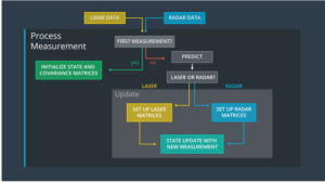
We try to achieve similar things with the Kalman filter and Unscented Kalman Filter processes. We two sensors and we wish to combine the information from both sensors (sensor fusion) but the different sensors produce different types of data and at different rates with different accuracy.
As you can see the UKF road map is a lot simpler than the Kalman Filter process.
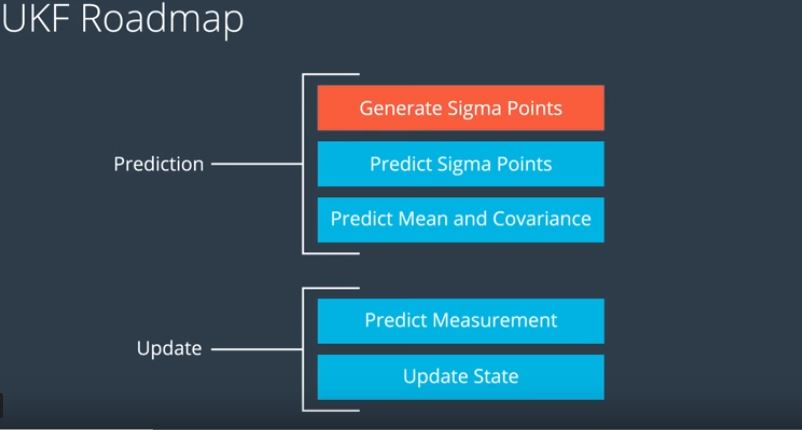
The essential difference between Kalman and unscented is the use of sigma points. I will attempt a short expatiation. Imagine you knew exact where something was and you plotted the exact spot on a map , you might say you pin pointed it. Meaning you can put the location with a high degree of certainty to a very small point. What if you are not so sure? Instead of a pin point you might have a bigger circle and say I am sure but the location is within this circle but I am not sure exactly where. The more uncertain you are the bigger the circle would be. Sigma points are made by taking the circle that represents the uncertainty and selecting a few points on it and using those instead of a perfect match to the entire circle surface or perimeter. This means we only have to do complex math for a few points and actually this is sufficiency accurate. The disadvantage of some loss of theoretical accuracy is offset by the fact that this technique works better on curves so it can outperform the Kalman filter in such circumstances.
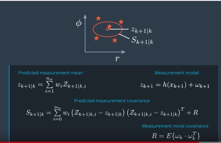
The above images show screenshots for the lectures as you can see plenty of hefty math to work through. Similar to the Kalman Filter we need to understand the equations enough to work with them and get them set up in a program but we don’t need to memorize them. We are still acting as Computer Engineers not Mathematicians.
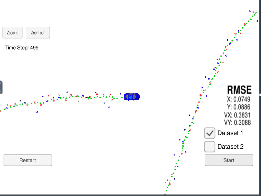
Also here we see the screen output when the program is running and similar to the Kalman filter project we have a little blue car and many coloured dots around it. The blue and red dots represent Radar and Lidar point and the Green dots represent a smoothed line that combins the detecions from Radar and Lidar.
Again like the Kalman filter I would say the picture is not as pretty or as dramatic as I would like. I feel like with all the effort I put in I would like to see something more spectacular but again like the Kalman filter this represents calculations that happen inside your car and may not have any usual output in normal use. Also I think the new version of the course has a nice output screen to look a little more exciting.
My outstanding impression of this project is that is was slightly easier than the Kalman Filter but both of these filters together represent the most challenging mathematics I have ever had to work with. It was great to be working on really tough material and to implement it in C++ was a great learning experience.


Functional Safety
Path Planning
PID
Particle Filter
Kalman Filter
